Spectral Clustering Algorithm

In this blog post, we’ll develop a simplified version of a spectral clustering algorithm that can be used to group complex distributions of data points.

This tutorial will be based on the template provided by Professor Phil Chodrow, which can be found in its entirety here.

Introduction

Suppose we have the following data points.

import numpy as np
from sklearn import datasets
from matplotlib import pyplot as plt

np.random.seed(1234)
n = 200
X, y = datasets.make_moons(n_samples=n, shuffle=True, noise=0.05, random_state=None)
plt.scatter(X[:,0], X[:,1])

<matplotlib.collections.PathCollection at 0x1af309e7a90>

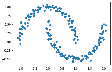
Visually, we can see that the points appear to be split into two groups. But how can we quantify these groups and label these points more explicitly, rather than just relying on a feeling of what it looks like?

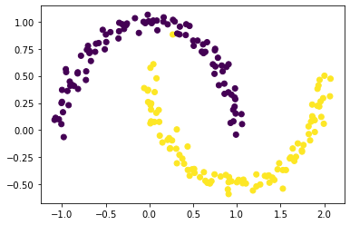
In this blog post, we will explore clustering, which refers to methods of grouping data points. One common clustering method is k-means, which tends to perform well on data points that form circular(-ish) blobs. For more complicated distributions of data points, however, k-means clustering falls apart. For instance, look at what happens when we apply k-means clustering to our crescent-moon data.

from sklearn.cluster import KMeans

km = KMeans(n_clusters = 2)
km.fit(X)
plt.scatter(X[:,0], X[:,1], c = km.predict(X))

<matplotlib.collections.PathCollection at 0x1af3134b340>

When we try applying k-means clustering, we get inaccurate representations, because these data points do not form the circular blobs that k-means clustering is equipped to handle. We will thus turn to spectral clustering instead, which is a useful tool that allows us to analyze data sets with complex structure and identify its most meaningful parts.

Part A

We begin by constructing a similary matrix A. A similarity matrix has the shape (n, n) (where n is the number of data points; in this case, 200), and entry A[i, j] equals 1 if X[i] (the coordinates of data point i) is within epsilon (which is some given value) distance of X[j] and 0 otherwise.

We can easily build our similarity matrix using the pairwise_distances function built into sklearn, which computes the distance matrix of a given vector (in our case, our vector of points X). After generating this distance matrix, we check pointwise if each distance is less than our desired epsilon, and convert the resulting boolean to an int. We save the resulting matrix in the variable A.

from sklearn.metrics import pairwise_distances

# in this case, we set epsilon = 0.4
epsilon = 0.4

A = (pairwise_distances(X) < epsilon).astype(int)
A

array([[1, 0, 0, ..., 0, 0, 0],
       [0, 1, 0, ..., 0, 0, 0],
       [0, 0, 1, ..., 0, 1, 0],
       ...,
       [0, 0, 0, ..., 1, 1, 1],
       [0, 0, 1, ..., 1, 1, 1],
       [0, 0, 0, ..., 1, 1, 1]])

We want all the diagonal entries A[i,i] to be equal to zero.

np.fill_diagonal(A, 0)
A

array([[0, 0, 0, ..., 0, 0, 0],
       [0, 0, 0, ..., 0, 0, 0],
       [0, 0, 0, ..., 0, 1, 0],
       ...,
       [0, 0, 0, ..., 0, 1, 1],
       [0, 0, 1, ..., 1, 0, 1],
       [0, 0, 0, ..., 1, 1, 0]])

Part B

We begin by writing a function for computing the cut term, which is the number of nonzero entries inA that relate points between the two clusters. We can calculate this cut term by summing the entries A[i, j] for each pair of points (i, j) in different clusters (i.e., by counting how many pairs of points in different clusters are within epsilon distance of each other).

def cut(A, y): 
    """
    Computes the cut term of a matrix A and 
    a cluster membership vector y. 
    
    @param A : the distance matrix. 
    @param y : the cluster membership vector.
    @return  : the cut term.
    """
    cut_term = 0
    
    for i in range(n):
        for j in range(n): 
            if y[i] != y[j]:
                cut_term += A[i][j]
    
    # we divide by 2 to 
    # account for double-counting
    return cut_term / 2 

We can now apply this function to our distance matrix A and our previously generated vector y, which notes the true clusters.

cut(A, y)

13.0

We now want to generate a random vector of random labels equal to either 0 or 1 (i.e., a random partition of our data points into one of the true clusters), and then check the cut objective for this random label vector.

random_label = np.random.randint(0, 2, size = n)
cut(A, random_label)

1136.0

As expected, we see that the cut term for these random labels is much, much higher. This makes sense intuitively–a small cut term indicates that the points in one cluster are not very close to the points in another cluster. In this case, the large cut term means that points between the two distinct clusters are close to each other, which in turn means that our clusters are probably entangled and not good ways of sorting our data into groups.

We now want to write a function to calculate the volume term. Recall that the volume of a cluster is a measure of how “big” that cluster is; more precisely, the volume of a cluster is the sum of the degrees of the rows of the data points in the cluster.

def vols(A, y):
    """
    Computes the volumes of 
    """
    # cluster 0
    vol0 = np.sum([np.sum(A[i]) for i in range(n) if y[i] == 0])
    
    # cluster 1
    vol1 = np.sum([np.sum(A[i]) for i in range(n) if y[i] == 1])
    
    return vol0, vol1

Finally, we can use our cut term and volume term functions to define a function that calculates the binary norm cut objective of a given matrix A.

def normcut(A, y):
    """
    """
    cut_term = cut(A, y)
    v0, v1 = vols(A, y)
    
    return cut_term * ( (1/v0) + (1/v1) )

Let us use this normcut function to generate objectives for both the true label y and the random labels random_label and see how they compare.

normcut(A, y)

0.011518412331615225

normcut(A, random_label)

1.0098636474944822

Recall that a pair of clusters is considered a good partition when the normcut is small. This is because the normcut is small when the cut term is small (i.e. the points in one cluster aren’t very close to another cluster; there is a notable distinction between the two clusters) and the volumes are large (so that neither partition is too small).

As expected, we see that the normcut is much higher (by a factor of approximately 100) for the random labels than the true labels.

Part C

We have now successfully defined the normcut, which can be used as a measure for how good a clustering is, since it takes on small values whenever the input clusters are joined by few entries and are not too small (i.e., the smaller the normcut the better). Thus, our first thought might be to try and find the set of cluster labels y that minimizes normcut(A, y). This, however, is a very hard problem, and can often not be computed in a practical amount of time. Thus, we turn our attention elsewhere.

Instead, we can define a vector z such that z_i equals the reciprocal of either vol(C_0) or -vol(C_1), depending on whether y_i = 0 or y_i = 1 (respectively). The cluster label for a given element i is contained in the sign of its associated element in z; if z_i is positive, then i must be in cluster 0, where as if z_i is negative, then i is from cluster 1.

Let’s write a function that will generate the z vector described above. We will call this function transform(A, y). It works using the formula described above, depending on the value of y_i.

def transform(A, y):
    z = np.zeros(n)
    vol0, vol1 = vols(A, y)
    
    for i in range(n): 
        if y[i] == 0:
            z[i] = 1/vol0
        else:
            z[i] = -1/vol1
             
    return z

We use the transform function we defined above on our data set to generate our z vector.

z = transform(A, y)
D = np.diag(np.sum(A, axis=0))

We also know that the normcut object is equal to the product of z.T and (D - A) and z divided by z.T times D times z. Let’s check that the z we generated above is properly related to the normcut:

RHS = (z @  (D - A) @ z)/(z @ D @ z)
LHS = normcut(A, y)
np.isclose(LHS, RHS)

True

As expected, we see that both sides of the equation are approximately equal.

While we’re at it, let’s also check the identity (i.e. z.T times D times the identity vector 1 equals 0).

one_vec = np.ones(n)

np.isclose(z @ D @ one_vec, 0)

True

We see that this too holds as desired.

Part D

As we saw in the previous part, the normcut is actually equal to z.T times (D - A) times z divided by z.T times D times z. Thus, we can actually minimize the normcut by minimimzing the aforementioned expression. Before we go to this step, however, let’s substitute the orthogonal complement of z relative to D1 in place of z. We want to do this because of the condition we mentioned above, the condition that z.T times D1 equals 0. We can do this using the orth_obj function, which was defined by Professor Chodrow below.

def orth(u, v):
    return (u @ v) / (v @ v) * v

e = np.ones(n) 

d = D @ e

def orth_obj(z):
    z_o = z - orth(z, d)
    return (z_o @ (D - A) @ z_o)/(z_o @ D @ z_o)

We can now use the minimize function from scipy.optimize in order to minimize orth_obj with respect to z. We will name the resulting minimizing vector z_min.

from scipy.optimize import minimize 

z_min = minimize(orth_obj, np.ones(n))
z_min = z_min.x

Part E

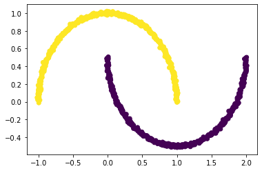
We know that the sign of z_min[i] is what contains information about which cluster a data point i is in. We thus plot our data, setting the points where z_min[i] < 0 to one color and the points where z_min[i] >= 0 to another color. The resulting scatter plot is a visualization of which clusters each of the points belongs to.

plt.scatter(X[:,0], X[:,1], c = (z_min >= 0))

<matplotlib.collections.PathCollection at 0x1af33acdd30>

There’s a few stragglers, but for the most part, it looks like we did a pretty good job clustering our data! The cluster colors match up with clusters that we would expect based on the data’s shape.

Part F

In reality, it’s usually too slow to always explicitly optimize the orthogonal objective, and so it’s not a practical option for spectral clustering. Luckily for us, there’s something else we can use: eigenvalues and eigenvectors.

Recall that we’re trying to minimize the normcut function, which we can do by minimizing the expression z.T times (D - A) times z divided by z.T times D times z (which is equal to the normcut, subjec to the condition that z.T times D1 equals 0). By the Rayleigh-Ritz Theorem, the minimizing z is the solution associated with the smallest eigenvalue of the following equation: (D - A) * z = lambda * Dz, with the condition that z.T * D1 = 0. This is equivalent to the problem D.inv * (D - A) * z = lambda * z, subject to the condition z.T * 1 = 0. This means that the eigenvector with the smallest eigenvalue is actually 1, and so our desired vector, z is the eigenvector that has the second-smallest eigenvalue.

We will thus first create a matrix L = D.inv * (D - A), also known as the Laplacian matrix of our similarity matrix A. We will then find the eigenvector that corresponds to its second-smallest eigenvalue and save it in the variable z_eig, whose sign we will use in turn to color our data plot.

D_inv = np.linalg.inv(D)
L = D_inv @ (D - A)

eigenvals, eigenvecs = np.linalg.eig(L)
eigenval_sort = eigenvals[np.argsort(eigenvals)]
eigenvec_sort = eigenvecs[:, np.argsort(eigenvals)]

# eigenvector associated with second smallest eigenvalue
z_eig = eigenvec_sort[:, 1]

plt.scatter(X[:,0], X[:,1], c = (z_eig <= 0))

<matplotlib.collections.PathCollection at 0x1af35f49160>

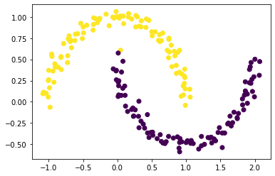
It worked pretty well! There’s one stray yellow dot in the realm of the purple, but it seems that everything else was clustered perfectly.

Part G

Our last step is to consolidate all of our results from the previous parts. We do so by writing a function called spectral_clustering(X, epsilon), which takes in some input data X and a distance threshold epsilon and then returns labels that indicate which cluster each data point is in. This function works exactly the way we computed clusters above: it first constructs the similarity matrix and fills its diagonals with zeros; it then constructs the Laplacian matrix; it the computes the eigenvector associated with the Laplacian matrix’s second-smallest eigenvalue; and finally, it uses this eigenvector to return an array of labels.

def spectral_clustering(X, epsilon):
    """
    Performs spectral clustering on a given set of data using a given distance threshold.
    @ param X: the given set of data. 
    @ param epsilon: the distance threshold.
    @ return: an array of labels that splits the original data into two clusters.
    """
    # 1. Construct the similarity matrix.
    A = (pairwise_distances(X) < epsilon).astype(int)
    np.fill_diagonal(A, 0)
    
    
    # 2. Construct the Laplacian matrix.
    D = np.diag(np.sum(A, axis=0))
    D_inv = np.linalg.inv(D)
    L = D_inv @ (D - A)
    
    
    # 3. Compute the eigenvector with the second-smallest 
    #    eigenvalue of the Laplacian matrix.
    eigenvals, eigenvecs = np.linalg.eig(L)
    eigenval_sort = eigenvals[np.argsort(eigenvals)]
    eigenvec_sort = eigenvecs[:, np.argsort(eigenvals)]
    z_eig = eigenvec_sort[:, 1]
    
    
    # Return labels based on this eigenvector. 
    labels = (z_eig <= 0)
    
    return labels

Now, let’s see this function in action! We use our same data and our same epsilon value and once again plot the results…

labels = spectral_clustering(X, epsilon)
plt.scatter(X[:,0], X[:,1], c = labels)

<matplotlib.collections.PathCollection at 0x1af34df5be0>

…and it works!

Part H

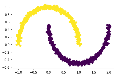
Now that we have a consolidated function that allows us to easily cluster points, let’s test this clustering out on different sets of data. We will generate several different data sets using the make_moons method, each with varying levels of noise, and see how our spectral clustering performs on each of them.

Noise = 0.01

n = 1000
X, y = datasets.make_moons(n_samples=n, shuffle=True, noise=0.01, random_state=None)
labels = spectral_clustering(X, epsilon)
plt.scatter(X[:,0], X[:,1], c = labels)

<matplotlib.collections.PathCollection at 0x1af362b3310>

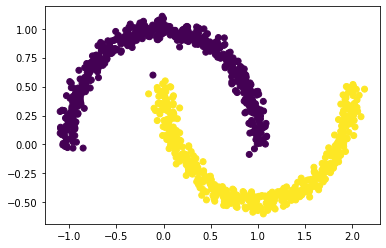
Noise = 0.03

n = 1000
X, y = datasets.make_moons(n_samples=n, shuffle=True, noise=0.03, random_state=None)
labels = spectral_clustering(X, epsilon)
plt.scatter(X[:,0], X[:,1], c = labels)

<matplotlib.collections.PathCollection at 0x1af3644dd30>

Noise = 0.05

n = 1000
X, y = datasets.make_moons(n_samples=n, shuffle=True, noise=0.05, random_state=None)
labels = spectral_clustering(X, epsilon)
plt.scatter(X[:,0], X[:,1], c = labels)

<matplotlib.collections.PathCollection at 0x1af363748e0>

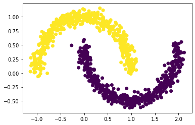
Noise = 0.07

n = 1000
X, y = datasets.make_moons(n_samples=n, shuffle=True, noise=0.07, random_state=None)
labels = spectral_clustering(X, epsilon)
plt.scatter(X[:,0], X[:,1], c = labels)

<matplotlib.collections.PathCollection at 0x1af364c1580>

Noise = 0.09

n = 1000
X, y = datasets.make_moons(n_samples=n, shuffle=True, noise=0.09, random_state=None)
labels = spectral_clustering(X, epsilon)
plt.scatter(X[:,0], X[:,1], c = labels)

<matplotlib.collections.PathCollection at 0x1af363e4550>

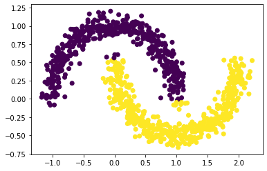
We notice that as we increase the noise, our data points get “fuzzier” and less compact. Regardless of the noise, however, our clustering algorithm works fairly well! For our first four plots, where the noise takes on values between 0.01 and 0.07, spectral_clustering is perfect; as we increase the noise to 0.09, we observe that our function has more difficulty with accurate clustering and mislabels some of the data points that are near the edges, but overall it still performs decently well.

Part I

We’ve worked a lot with the half-moon shapes; now let’s try another shape–the bull’s eye–to make sure that our spectral_clustering algorithm is robust. We generate our data points using the make_circles function and plot the resulting bull’s eye shape.

n = 1000
X, y = datasets.make_circles(n_samples=n, shuffle=True, noise=0.05, random_state=None, factor = 0.4)
plt.scatter(X[:,0], X[:,1])

<matplotlib.collections.PathCollection at 0x1af33943580>

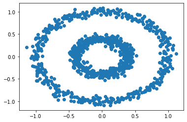
The plot shows two concentric circles. If we try to apply k-means clustering to these points, we don’t get a satisfactory result:

km = KMeans(n_clusters = 2)
km.fit(X)
plt.scatter(X[:,0], X[:,1], c = km.predict(X))

<matplotlib.collections.PathCollection at 0x1af34dfd610>

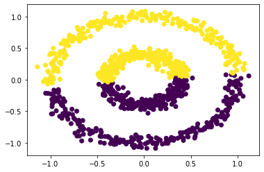
Let’s try spectral clustering instead, and play around with different values of epsilon. This is not pictured below, but is easily done by changing the epsilon argument of the spectral_clustering method.

labels = spectral_clustering(X, epsilon = 0.52)
plt.scatter(X[:,0], X[:,1], c = labels)

<matplotlib.collections.PathCollection at 0x1af36244b20>

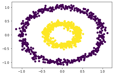
After testing many different epsilon values between 0 and 1.0, we find that our function works successfully for values of epsilon roughly between 0.21 and 0.52 (inclusive).